REED: You Can Calculate Power Retrospectively — Just Don’t Use Observed Power

Last updated on Nov 5, 2025

In this blog, I highlight a valid approach for calculating power after estimation—often called retrospective power. I provide a Shiny App that lets readers explore how the method works and how it avoids the pitfalls of “observed power” — try it out for yourself! I also link to a webpage where readers can enter any estimate, along with its standard error and degrees of freedom, to calculate the corresponding power.

A. Why retrospective power can be useful

Most researchers calculate power before estimation, generally to plan sample sizes: given a hypothesized effect, a significance level, and degrees of freedom, power analysis asks how large a study must be to achieve a desired probability of detection.

That’s good practice, but key inputs—variance, number of clusters, intraclass correlation coefficient (ICC), attrition, covariate performance—are guessed before the data exist, so realized (ex post) values often differ from what was planned. As Doyle & Feeney (2021) note in their guide to power calculations, “the exact ex post value of inputs to power will necessarily vary from ex ante estimates.” This is why it can be useful—even preferable—to also calculate power after estimation.

Ex-post power can be helpful in at least three situations.

It can provide a check on whether ex-ante power assessments were realized. Because actual implementation rarely matches the original plan—fewer participants recruited, geographic constraints on clusters, or greater dependency within clusters than anticipated—realized power often departs from planned power. Calculating ex-post power highlights these gaps and helps diagnose why they occurred.
It can help distinguish whether a statistically insignificant estimate reflects a negligible effect size or an imprecise estimate. In other words, it can separate “insignificant because small” from “insignificant because underpowered.”
It can flag potential Type M (magnitude) risk when results are significant but measured power is low. In this way, it can warn of possible overestimation and prompt more cautious interpretation ( Gelman & Carlin, 2014).

In short, while ex-ante power is essential for planning, ex-post power is a practical complement for evaluation and interpretation. It connects power claims with realized outcomes, enables the diagnosis of deviations from plan, and provides additional insights when interpreting both null and significant findings.

B. Why the usual way (“Observed Power”) is a bad idea

Most statisticians advise against computing observed power, which plugs the observed effect and its estimated standard error into a power formula ( McKenzie & Ozier, 2019). Because observed power is a one-to-one (monotone) transformation of the test statistic—and hence of the p-value—it adds no information and encourages tautological explanations (e.g., “the result was non-significant because power was low”).

Worse, as an estimator of a study’s design power, observed power is both biased and high variance, precisely because it treats a noisy point estimate as the true effect. These problems are well documented ( Hoenig & Heisey, 2001; Goodman & Berlin, 1994; Cumming, 2014; Maxwell, Kelley, & Rausch, 2008). These concerns are not just theoretical: I demonstrate below how minor sampling variation translates into dramatic changes in observed power.

C. A better retrospective approach: SE–ES

In a recent paper ( Tian et al., 2024), I and my coauthors propose a practical alternative that we call: SE–ES (Standard Error–Effect Size). The idea is simple. The researcher specifies a hypothesized effect size (what would be substantively important), uses the estimated standard error from the fitted regression, and combines those with the relevant degrees of freedom to compute power for a two‑sided t‑test.

Because SE–ES fixes the effect size externally—rather than using the noisy point estimate—it yields a serviceable retrospective power number: approximately unbiased for the true design power with a reasonably tight 95% estimation interval, provided samples are not too small.

To make this concrete, suppose the data-generating process is Y=a+bX+ε , with ε a classical error term and b estimated by OLS. If the true design power is 80%, simulations at sample sizes n = 30, 50, 100 show that the SE–ES estimator is approximately unbiased, with 95% estimation intervals that tighten as n grows: (i) n = 30 yields (60%, 96%); (ii) n = 50 yields (65%, 94%); and (iii) n = 100 yields (70%, 90%).

D. Try it yourself: A Shiny app that compares SE–ES with Observed Power

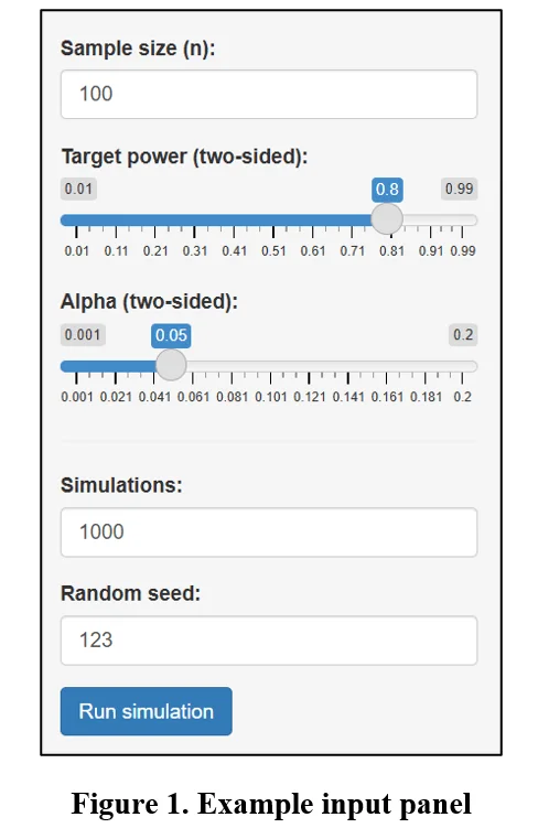
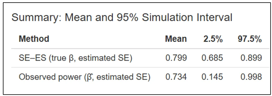
To visualize the contrast, I have created a companion Shiny app. It lets you vary sample size (n), target/true power, and α, then: (1) runs Monte Carlo replications of Y ~ 1 + βX; (2) plots side‑by‑side histograms of retrospective power for SE–ES and Observed Power; and (3) reports the Mean and the 95% simulation interval (the central 2.5%–97.5% range of simulated power values) for each method. Power is calculated under two‑tailed testing.

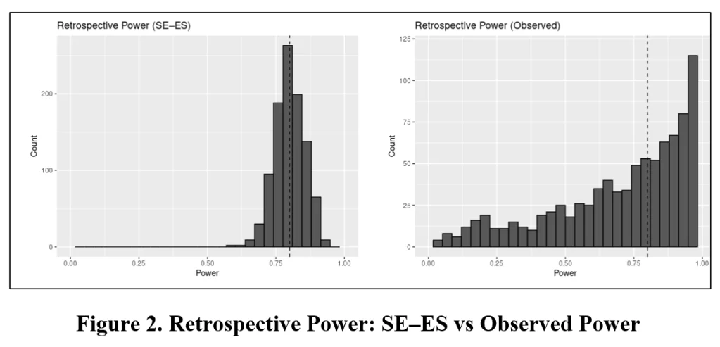
What you should see: the Observed Power histogram tracks the significance test—mass near 0 when results are null, near 1 when they are significant—because it is just a re‑expression of the t statistic. Further, the wide range of estimates makes it unusable even if its biasedness did not. The SE–ES histogram, in contrast, concentrates near the design’s target power and tightens as sample size grows.

To use the app, click here. Input the respective values in the Shiny app’s sidebar panel. The panel below provides an example with sample size set equal to 100; true power equal to 80% (for two-sided significance), alpha equal to 5%, and sets the number of simulations = 1000 and the random seed equal to 123.

Once you have entered your input values, click “Run simulation”. Two histograms will appear. The histogram to the left reports the distribution of estimated power values using the SE-ES method. The histogram to the right reports the same using Observed Power. The vertical dotted line indicates true power.

Immediately below this figure, the Shiny app produces a table that reports the mean and 95% estimation interval of estimated powers for the SE-ES and Observed Power methods. For this example, with the true power = 80%, the Observed Power distribution is left skewed, biased downwards (mean = 73.4%) with a 95% estimation interval of (14.5%, 99.8%). In contrast, the SE-ES distribution is approximately symmetric, approximately centered around the true of 80%, with a 95% estimation interval of (68.5%, 89.9%).

The reader is encouraged to try out different target power values and, most importantly, sample sizes. What you should see is that the SE-ES method works well at every true power value, but, in this context, it becomes less serviceable for sample sizes below 30.

E. Bottom line—and an easy calculator you can use now

Power estimation is useful for before estimation, for planning. But it is also useful after estimation, as an interpretative tool. Furthermore, it is easy to calculate. For readers interested in calculating retrospective power for their own research, Thomas Logchies and I have created an online calculator that is easy to use: click here. There you can enter α, degrees of freedom, an estimated standard error, and a hypothesized effect size to obtain SE–ES retrospective power for your estimate. Give it a go!

NOTE: Bob Reed is Professor of Economics and the Director of UCMetaat the University of Canterbury. He can be reached at bob.reed@canterbury.ac.nz.

References

Cumming, G. (2014). The new statistics: Why and how. Psychological Science, 25(1), 7–29. https://doi.org/10.1177/0956797613504966

Doyle, M.-A., & Feeney, L. (2021). Quick guide to power calculations. https://www.povertyactionlab.org/resource/quick-guide-power-calculations

Gelman, A., & Carlin, J. (2014). Beyond power calculations: Assessing type S (sign) and type M (magnitude) errors. Perspectives on Psychological Science, 9(6), 641–651. https://sites.stat.columbia.edu/gelman/research/published/retropower_final.pdf

Goodman, S. N., & Berlin, J. A. (1994). The use of predicted confidence intervals when planning experiments and the misuse of power when interpreting results. Annals of Internal Medicine, 121(3), 200–206. https://doi.org/10.7326/0003-4819-121-3-199408010-00008

Hoenig, J. M., & Heisey, D. M. (2001). The abuse of power: The pervasive fallacy of power calculations for data analysis. The American Statistician, 55(1), 19–24. https://doi.org/10.1198/000313001300339897

Maxwell, S. E., Kelley, K., & Rausch, J. R. (2008). Sample size planning for statistical power and accuracy in parameter estimation. Annual Review of Psychology, 59(1), 537–563. https://doi.org/10.1146/annurev.psych.59.103006.093735

McKenzie, D., & Ozier, O. (2019, May 16). Why ex-post power using estimated effect sizes is bad, but an ex-post MDE is not. Development Impact (World Bank Blog). https://blogs.worldbank.org/en/impactevaluations/why-ex-post-power-using-estimated-effect-sizes-bad-ex-post-mde-not

Tian, J., Coupé, T., Khatua, S., Reed, W. R., & Wood, B. D. (2025). Power to the researchers: Calculating power after estimation. Review of Development Economics, 29(1), 324-358. https://doi.org/10.1111/rode.13130

Like Loading…